The California Current
merged satellite-derived 4-km dataset for the CalCOFI region
Mati Kahru, mkahru@ucsd.edu Updated : May 13, 2018
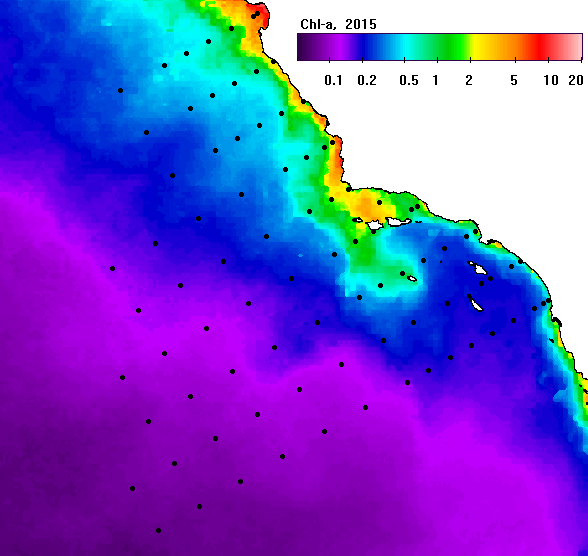
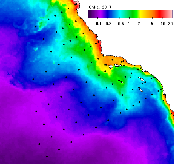
Satellite ocean color data from all available satellites are processed with regionally optimized Chlorophyll-a (Chla) algorithms fitted to a large dataset of in situ measurements[Kahru et al. 2012, Trends in the surface chlorophyll of the California Current: Merging data from multiple ocean color satellites, Deep-Sea Research. II, 77-80, 89-98; PDF); Kahru et al. 2015, Optimized merger of ocean chlorophyll algorithms, IEEE Geoscience and Remote Sensing Letters, 12, 11; PDF). The time series start with OCTS (Nov., 1996) and are followed by SeaWiFS (1997-2010), MERIS (2002-2012), MODISA (2002-present) and VIIRS (2012-present). Daily spectral remote sensing reflectance (Rrs) data at 4 km resolution (9 km for OCTS and SeaWiFS) are used to calculate daily products for each sensor after which overlapping datasets are merged. Note that this is different from the 1-km data merger products that are available at http://www.wimsoft.com/CAL/. The 1-km products are merged between the standard products and without applying the regionally optimized algorithms to the Rrs. The 4-km daily datasets are mapped to a grid with 1.5 km resolution and composited into 5-day products with missing pixels filled with temporal interpolation between the previous and the next 5-day product. The interpolation procedure is applied twice. The interpolated 5-day datasets are used to create 15-day and monthly composites and the monthly composites are then used to create annual composites. For each period the corresponding anomalies are created as ratios to the longterm mean annual cycle (1996/Nov to present). The following example shows the recovery in Chla from the lows in 2015 to 2017.
|
|
|
|
|
|
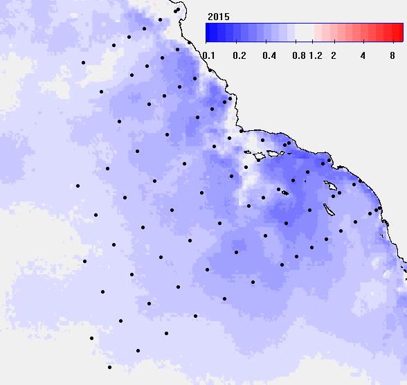

Fig. 1. An example of annual mean Chla for 2015 (upper left), 2017 (upper right) and the respective anomales (lower panels) as ratios to the longterm mean. In the anomaly images the blue colors represent significant reduction and the red colors represent significant increase with white meaning no significant change (at 95% significance).
The anomaly panels show that in 2015 the most of area was significantly (95%) below longterm mean (blue) with some areas (white) not significantly different from normal. In 2017 the central California upwelling area had turned significantly above the longterm mean (pink) while other regions (blue) still remained below the longterm mean.
5-day interpolated, 15-day, monthly and annual products are zipped together in both PNG or JPG and HDF4 formats. PNG/JPG files are easy to visualize while the HDF4 files can be used to quantitativey extract pixel values. For each dataset the respective anomalies are also provided as zipped PNG and HDF4 files.
The datasets are in Zipped files and can be downloaded using the following hyperlinks:
|
PNG of Chla |
HDF4 of Chla |
JPG of Chla Anomaly |
HDF4 of Chla Anomaly |
For each cruise we can calculate the Mean Chla composite for the observation period (e.g. , 28-Mar-2015 to 26-Apr-2015 for cruise 201502), the interannual Mean for the same time period (e.g. 28-Mar to 26-Apr) over all available years, and the ratio of the current period mean to the longterm mean. The ratio to the longterm Mean is uased as a measure of the anomaly. These datasets in both HDF4 and PNG formats are zipped and available for downloading in the Table below.
|
Cruise |
Cruise |
Cruise |
Cruise |
The datasets on a grid of 588 (width) x 566 (height) with approximately 1500 m step are in HDF4 format. The upper-left corner (lat, lon) is 37N; -126.125E; the lower-right corner is 29.51349N; -116.6828E. Chla values in each pixel of unsigned byte are log10-scaled and can be calculated from the pixel value (PV) as: Chl (mg m-3) = 10^(0.015 * PV - 2.0), i.e. 10 to the power of 0.015 * PV - 2.0. Pixel values 0, 1 (black in Fig. 1) and 255 (white in Fig. 1) are considered invalid and must be excluded from any statistics. PV = 1 is used for coastline and has to be excluded too. The annotation (color bar) is written into the dataset. When reading with Matlab the unsigned byte variable is sometimes reported as signed byte (int8, values from -127 to 128) and not as unsigned byte (values from 0 to 255) and values over 128 become negative. A simple fix is to add 256 if the signed pixel value is negative. Anomaly images are linearly scaled byte images with the middle pixel value 128 corresponding to anomaly=1, i.e. no ratio anomaly. The scale ad intercept can be read from the HDF attributes.